Holycow - Advance Plots with R

My recent Holycow articles on Valeant and Wirecard followed the same pattern blurb, chart price with event annotations, chart volume, chart market cap. This article demonstrates how its done.

Load required libraries

knitr::opts_chunk$set(echo = TRUE)
require(tidyquant)
require(tidyverse)
library(ggplot2)
library(gridExtra)
library(grid)
library(cowplot)

Point to folder containing csvs (to annotate price info) and images.

folder <- "/folder/containing/csv/data"

Retrieve the stock price

All the report data will be organised in simple list structure called hc (holycow). Tidyquant will be used to retrieve price information. For demonstration I will work with Bausch which has a stock symbol BHC.

hc <- list()
hc$price <- tq_get("BHC", get = "stock.prices", from = "2000-01-01", to = "2020-06-26")

Prepare the annotations

A. Read the annotations (events) from a CSV.

# Get the annotations from csv and add price information for positioning
hc$eventsFile <- paste(folder, "/valeant_events.csv", sep="")
hc$events<-read_csv(  hc$eventsFile )

What is in that CSV?

hc$events %>% knitr::kable()

event	date
Hillary tweets about Valeant price gouging	21/09/2015
CEO resignation	21/03/2016

B. Add geometry data

For each event we need to add cartesian coordinates. GGPlot makes this relatively easy by mapping the coordinates to the graph data. In this case x will map to date and y maps to price.

The events source has the date with each event description, so we have the x already. We need to add the price for the y. To accomplish this I use dplyr join. It will need to join using the date field, as this field has the same name “date” in both sides of the join, and its the only common column, we dont need to give it a mapping, otherwise use the by argument inner_join(right, by(“somedate” = “someotherdate”)). However the datatype of the date field will have to be treated so that both date fields have same type.

# Get the annotations from csv and add price information for positioning

hc$events %>% 
  mutate(date=as.Date(parse_date_time(date,orders = c("dmy", "mdy", "ymd")))) %>% 
  inner_join(hc$price) -> 
  hc$events

## Joining, by = "date"

Prevent clipping of annotations

Some crude preperation of limits which will be used to add space to the chart. In this particular case only the y needs a bump, but it allows for x anyway. n1 is axis data floor, n2 is axis data max, n3 is axis extended amount.

hc$limits<-list()
hc$limits$x1 <- hc$price$date[1]
hc$limits$x2 <- hc$price$date[nrow(hc$price)]
hc$limits$x3 <- hc$limits$x2 + (0)
hc$limits$y1 <- 0
hc$limits$y2 <- hc$price$close[nrow(hc$price)]
hc$limits$y3 <- hc$limits$y2 + 300

Just draw the damn plots already

# chart Price
hc$price %>%
  ggplot() +
  geom_line(aes(x = date, y = close)) +
  labs(title = "Valiant Volume and price", y = "Closing Price", x = "") + 
  geom_point(data=hc$events, aes(x=date, y=close, color="red"), show.legend = FALSE) +
  geom_text(data=hc$events, aes(x=date+100, y=close+10,label=event), hjust="left", size=2, angle=22, color="blue") +
  expand_limits(x = c(hc$limits$x1, hc$limits$x3), y = c(hc$limits$y1, hc$limits$y3)) +
  theme_tq() + 
  theme(plot.margin = margin(b=0, unit="pt")) ->
  hc$chartPrice

# chart Volume
hc$price %>%
  mutate (volume = volume/1000000) %>%
  ggplot(aes(x = date, y = volume)) +
  geom_segment(aes(xend = date, yend = 0, color = volume)) + 
  geom_smooth(method = "loess", se = FALSE, formula = y ~ x) +
  labs(
       y = "Volume", x = "") +
  expand_limits(x = c(hc$limits$x1, hc$limits$x3)) +
  theme_tq() +
  theme(legend.position = "none", plot.margin = margin(t=0, unit="pt"))  ->
  hc$chartVolume

# plot_grid comes from the cowplot library
plot_grid(hc$chartPrice, hc$chartVolume, align = "v", nrow = 2, rel_heights = c(4, 2))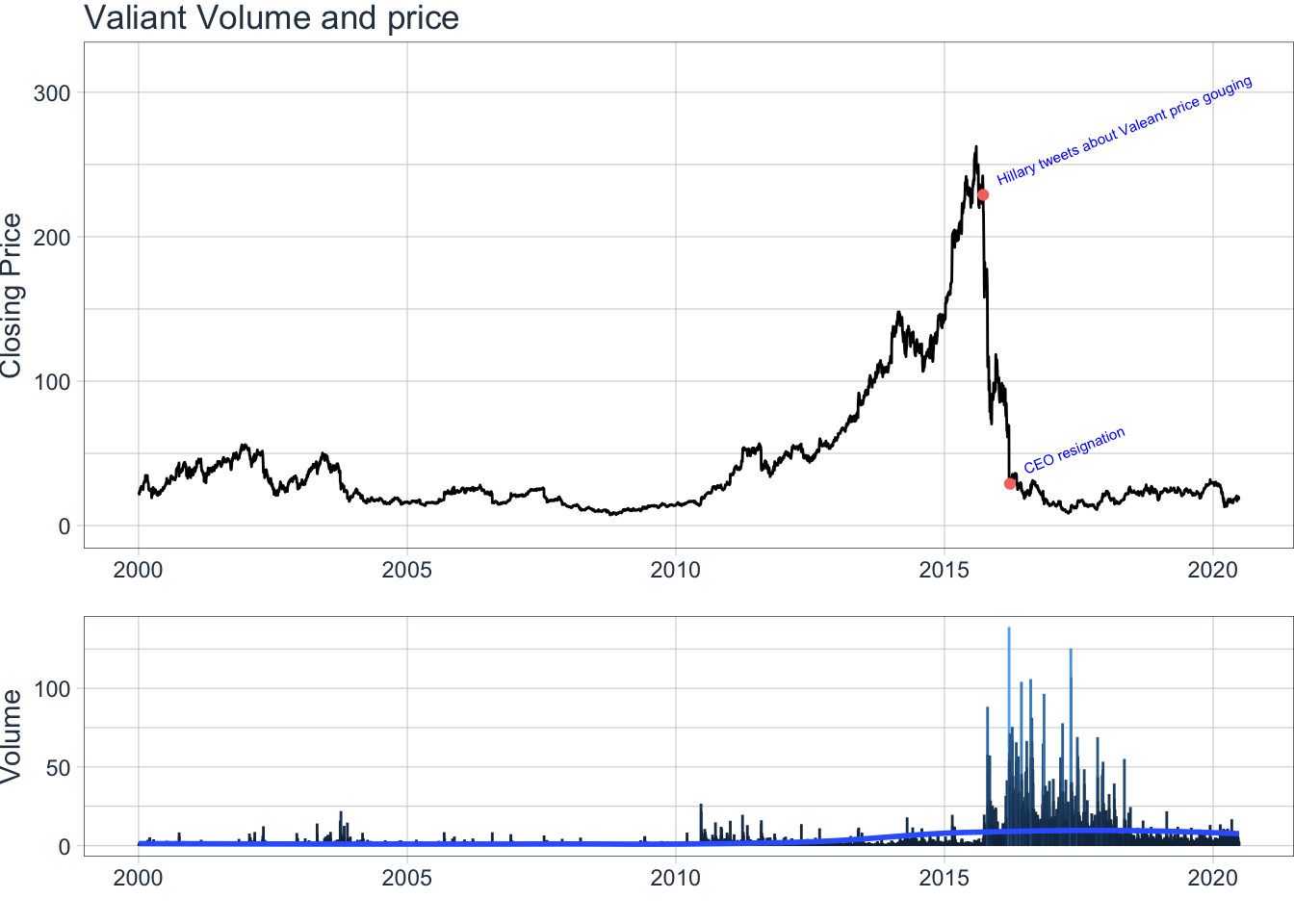

Notes

What happend to market cap? I dont have a free source for market cap data, I don’t have the right to distribute the data, and it would not add any value to this demonstration, so I have ommitted it from this howto.

What does the -> operator do? Forgive me for this, its an assignment operator with the opposite direction from the familiar assignment operators (<-, =). I like to use rarely seen operator alongside dplyr’s pipe operator for asthetic reasons, keeping the flow consistent, and/or just to be awkward.